mlair.plotting.postprocessing_plotting
Collection of plots to evaluate a model, create overviews on data or forecasts.
Module Contents
Classes
Show a monthly summary over all stations for each lead time (“ahead”) as box and whiskers plot. |
|
Create cond.quantile plots as originally proposed by Murphy, Brown and Chen (1989) [But in log scale]. |
|
Create plot of climatological skill score after Murphy (1988) as box plot over all stations. |
|
Create competitive skill score plot. |
|
Create plot of feature importance analysis. |
|
Create time series plot. |
|
Abstract class for all plotting routines to unify plot workflow. |
|
Abstract class for all plotting routines to unify plot workflow. |
|
Abstract class for all plotting routines to unify plot workflow. |
|
Abstract class for all plotting routines to unify plot workflow. |
|
Abstract class for all plotting routines to unify plot workflow. |
Attributes
-
mlair.plotting.postprocessing_plotting.__date__= 2020-11-23
-
class
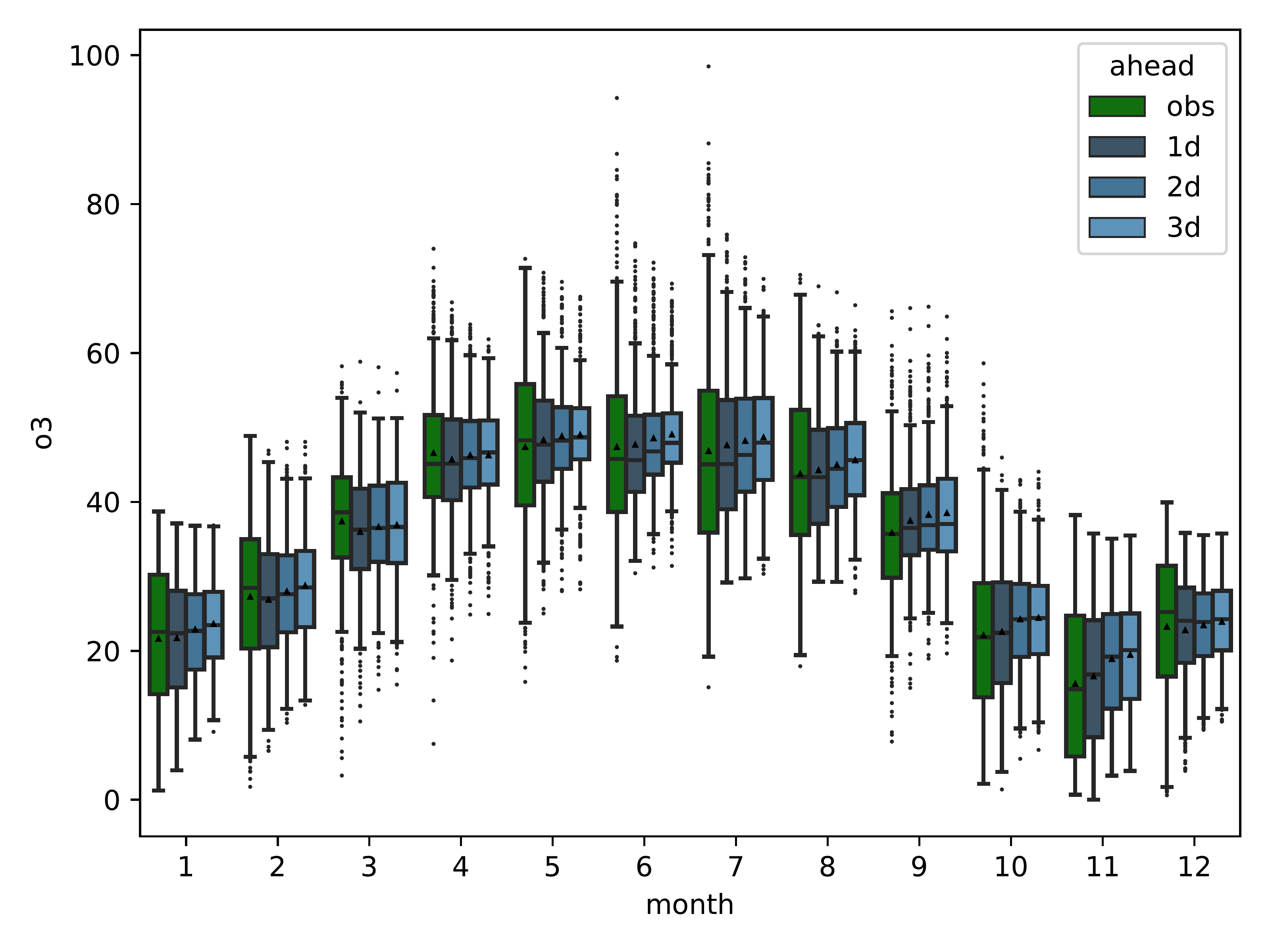
mlair.plotting.postprocessing_plotting.PlotMonthlySummary(stations: List, data_path: str, name: str, target_var: str, window_lead_time: int = None, plot_folder: str = '.', target_var_unit: str = 'ppb', model_name='nn')¶ Bases:
mlair.plotting.abstract_plot_class.AbstractPlotClassShow a monthly summary over all stations for each lead time (“ahead”) as box and whiskers plot.
The plot is saved in data_path with name monthly_summary_box_plot.pdf and 500dpi resolution.
- Parameters
stations – all stations to plot
data_path – path, where the data is located
name – full name of the local files with a % as placeholder for the station name
target_var – display name of the target variable on plot’s axis
window_lead_time – lead time to plot, if window_lead_time is higher than the available lead time or not given the maximum lead time from data is used. (default None -> use maximum lead time from data).
plot_folder – path to save the plot (default: current directory)
target_var_unit – unit of target var for plot legend (default= ppb)
-
_prepare_data(self, stations: List) → xarray.DataArray¶ Pre.process data required to plot.
For each station, load locally saved predictions, extract the CNN prediction and the observation and group them into monthly bins (no aggregation, only sorting them).
- Parameters
stations – all stations to plot
- Returns
The entire data set, flagged with the corresponding month.
-
_get_window_lead_time(self, window_lead_time: int)¶ Extract the lead time from data and arguments.
If window_lead_time is not given, extract this information from data itself by the number of ahead dimensions. If given, check if data supports the give length. If the number of ahead dimensions in data is lower than the given lead time, data’s lead time is used.
- Parameters
window_lead_time – lead time from arguments to validate
- Returns
validated lead time, comes either from given argument or from data itself
-
class
mlair.plotting.postprocessing_plotting.PlotConditionalQuantiles(stations: List, data_pred_path: str, plot_folder: str = '.', plot_per_seasons=True, rolling_window: int = 3, forecast_indicator: str = 'nn', obs_indicator: str = 'obs', competitors=None, model_type_dim: str = 'type', index_dim: str = 'index', ahead_dim: str = 'ahead', competitor_path: str = None, sampling: str = 'daily', model_name: str = 'nn', **kwargs)¶ Bases:
mlair.plotting.abstract_plot_class.AbstractPlotClassCreate cond.quantile plots as originally proposed by Murphy, Brown and Chen (1989) [But in log scale].
Link to paper: https://journals.ametsoc.org/doi/pdf/10.1175/1520-0434%281989%29004%3C0485%3ADVOTF%3E2.0.CO%3B2
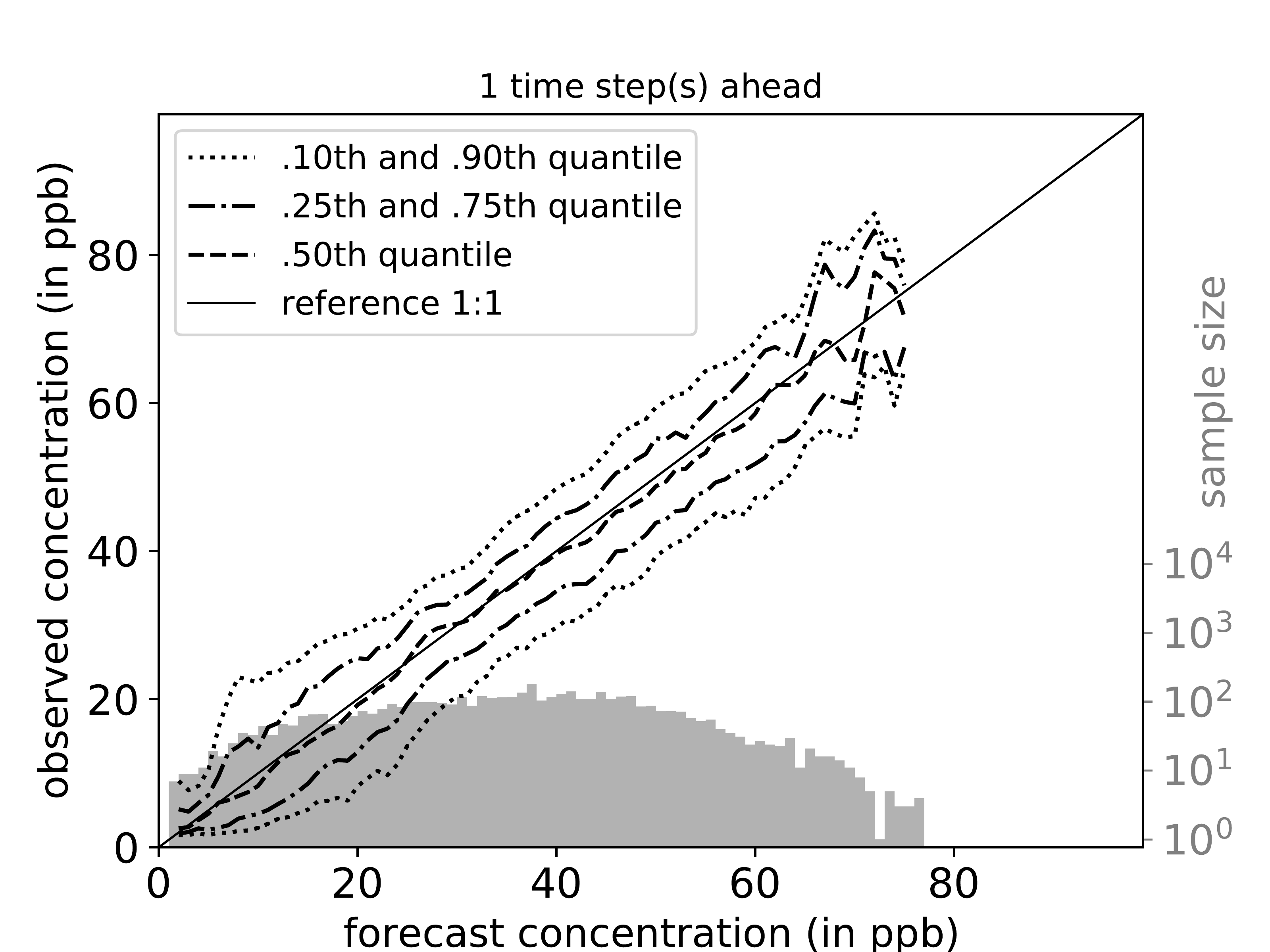
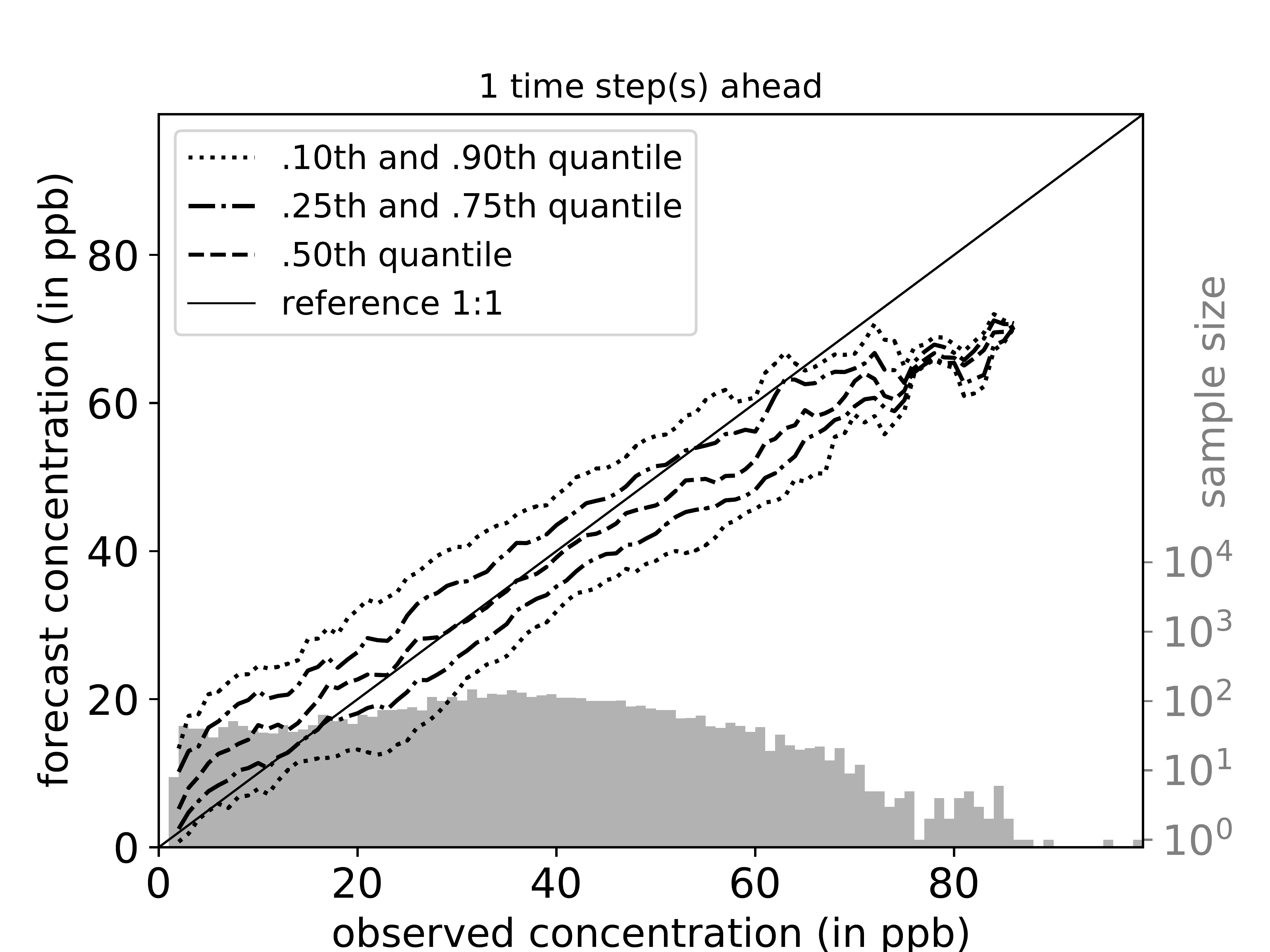
For each time step ahead a separate plot is created. If parameter plot_per_season is true, data is split by season and conditional quantiles are plotted for each season in addition.
- Parameters
stations – all stations to plot
data_pred_path – path to dir which contains the forecasts as .nc files
plot_folder – path where the plots are stored
plot_per_seasons – if `True’ create cond. quantile plots for _seasons (DJF, MAM, JJA, SON) individually
rolling_window – smoothing of quantiles (3 is used by Murphy et al.)
model_name – name of the model prediction as stored in netCDF file (for example “nn”)
obs_name – name of observation as stored in netCDF file (for example “obs”)
kwargs – Some further arguments which are listed in self._opts
-
static
_get_opts(kwargs)¶ Extract options from kwargs.
-
_load_data(self) → xarray.DataArray¶ Load plot data.
- Returns
plot data
-
_combine_forecasts(self, forecast, competitor, dim=None)¶ Combine forecast and competitor if both are xarray. If competitor is None, this returns forecasts and vise versa.
-
load_competitors(self, station_name: str, start, end) → xarray.DataArray¶ Load all requested and available competitors for a given station. Forecasts must be available in the competitor path like <competitor_path>/<target_var>/forecasts_<station_name>_test.nc. The naming style is equal for all forecasts of MLAir, so that forecasts of a different experiment can easily be copied into the competitor path without any change.
- Parameters
station_name – station indicator to load competitors for
- Returns
a single xarray with all competing forecasts
-
static
create_full_time_dim(data, dim, sampling, start, end)¶ Ensure time dimension to be equidistant. Sometimes dates if missing values have been dropped.
-
_create_competitor_forecast(self, station_name: str, competitor_name: str, start, end) → xarray.DataArray¶ Load and format the competing forecast of a distinct model indicated by competitor_name for a distinct station indicated by station_name. The name of the competitor is set in the type axis as indicator. This method will raise either a FileNotFoundError or KeyError if no competitor could be found for the given station. Either there is no file provided in the expected path or no forecast for given competitor_name in the forecast file. Forecast is trimmed on interval start and end of test subset.
- Parameters
station_name – name of the station to load data for
competitor_name – name of the model
- Returns
the forecast of the given competitor
-
static
_correct_persi_name(competitors)
-
_segment_data(self, data: xarray.DataArray, x_model: str) → xarray.DataArray¶ Segment data into bins.
- Parameters
data – data to segment
x_model – name of x dimension
- Returns
segmented data
-
static
_labels(plot_type: str, data_unit: str = 'ppb') → Tuple[str, str]¶ Assign (x,y) labels to plots correctly, depending on like-base or cali-ref factorization.
- Parameters
plot_type – type of plot, either obs or a model name
data_unit – unit of data to add to labels (default ppb)
- Returns
tuple with y and x labels
-
_get_bins_from_rage_of_data(self) → numpy.ndarray¶ Get array of bins to use for quantiles.
- Returns
range from 0 to data’s maximum + 1 (rounded down)
-
_create_quantile_panel(self, data: xarray.DataArray, x_model: str, y_model: str) → xarray.DataArray¶ Calculate quantiles.
- Parameters
data – data to calculate quantiles
x_model – name of x dimension
y_model – name of y dimension
- Returns
quantile panel with binned data
-
static
add_affix(affix: str) → str¶ Add additional information to plot name with leading underscore or add empty string if affix is empty.
- Parameters
affix – string to add
- Returns
affix with leading underscore or empty string.
-
_prepare_plots(self, data: xarray.DataArray, x_model: str, y_model: str) → Tuple[xarray.DataArray, xarray.DataArray]¶ Get segmented data and quantile panel.
- Parameters
data – plot data
x_model – name of x dimension
y_model – name of y dimension
- Returns
segmented data and quantile panel
-
_plot(self)¶ Start plotting routines: overall plot and seasonal (if enabled).
-
_plot_seasons(self)¶ Create seasonal plots.
-
_plot_all(self)¶ Plot overall conditional quantiles on full data.
-
class
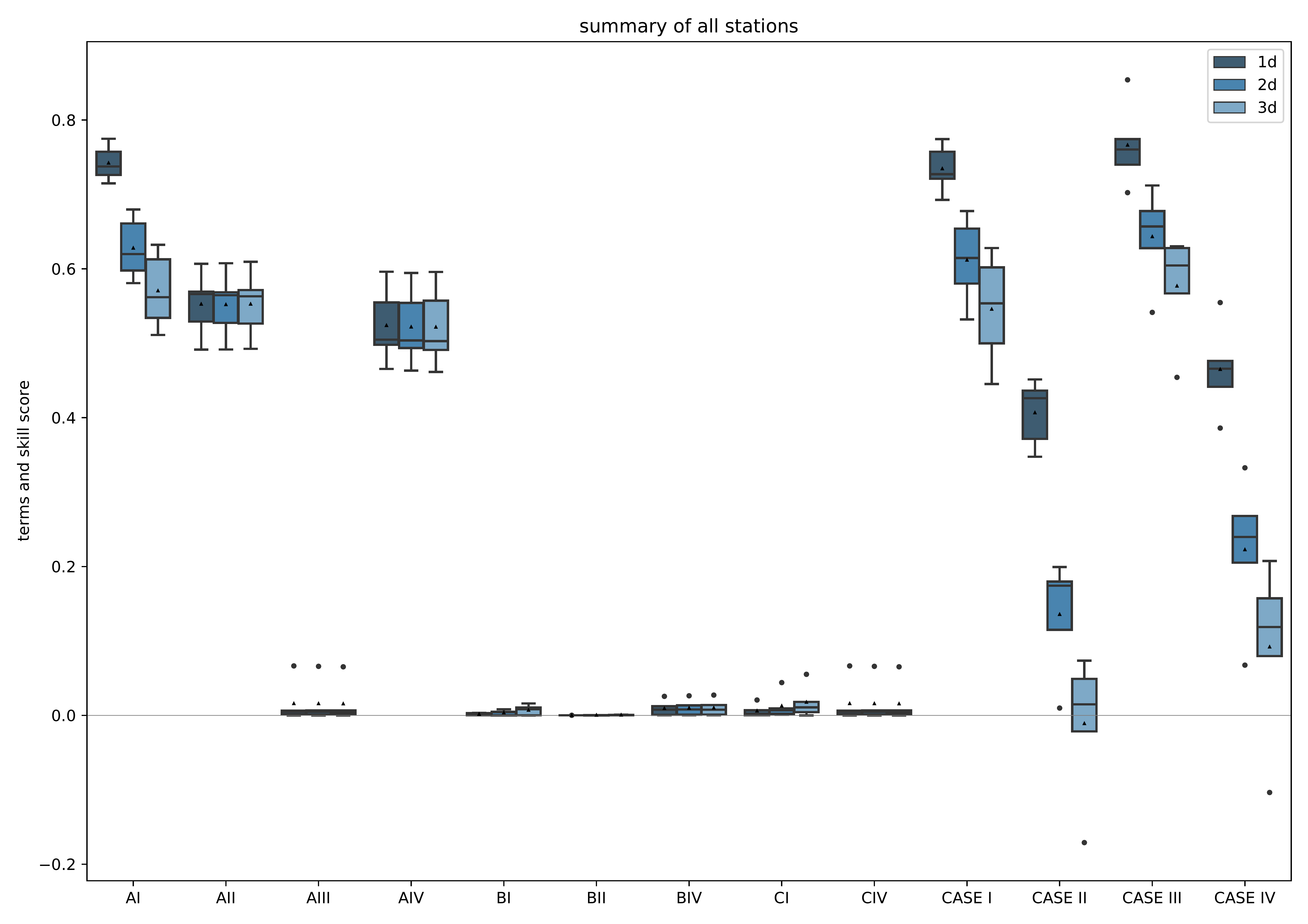
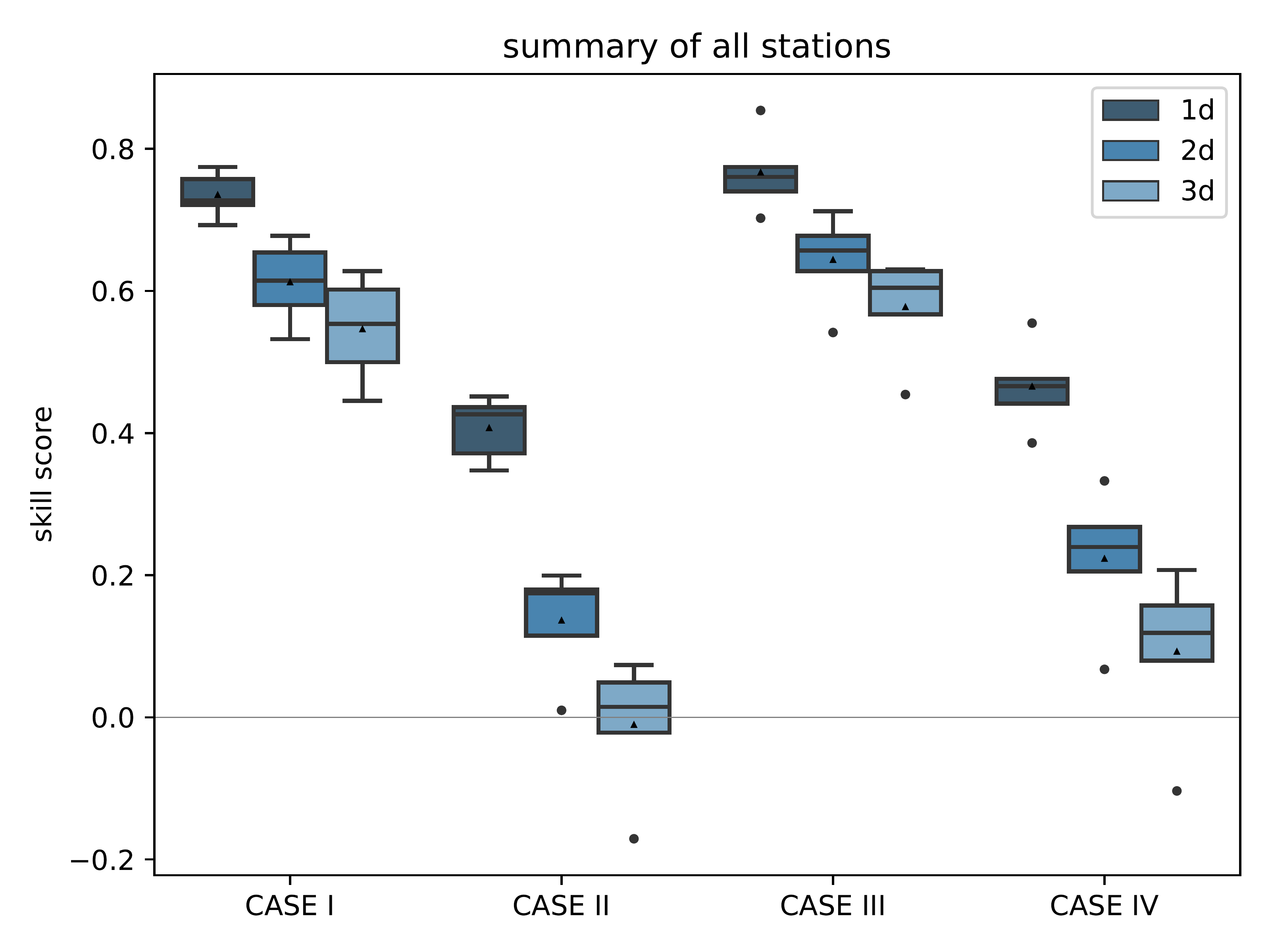
mlair.plotting.postprocessing_plotting.PlotClimatologicalSkillScore(data: Dict, plot_folder: str = '.', score_only: bool = True, extra_name_tag: str = '', model_name: str = '')¶ Bases:
mlair.plotting.abstract_plot_class.AbstractPlotClassCreate plot of climatological skill score after Murphy (1988) as box plot over all stations.
A forecast time step (called “ahead”) is separately shown to highlight the differences for each prediction time step. Either each single term is plotted (score_only=False) or only the resulting scores CASE I to IV are displayed (score_only=True, default). Y-axis is adjusted following the data and not hard coded. The plot is saved under plot_folder path with name skill_score_clim_{extra_name_tag}{model_setup}.pdf and resolution of 500dpi.
- Parameters
data – dictionary with station names as keys and 2D xarrays as values, consist on axis ahead and terms.
plot_folder – path to save the plot (default: current directory)
score_only – if true plot only scores of CASE I to IV, otherwise plot all single terms (default True)
extra_name_tag – additional tag that can be included in the plot name (default “”)
model_name – architecture type to specify plot name (default “”)
-
_prepare_data(self, data: Dict, score_only: bool) → pandas.DataFrame¶ Shrink given data, if only scores are relevant.
In any case, transform data to a plot friendly format. Also set plot labels depending on the lead time dimensions.
- Parameters
data – dictionary with station names as keys and 2D xarrays as values
score_only – if true only scores of CASE I to IV are relevant
- Returns
pre-processed data set
-
_label_add(self, score_only: bool)¶ Add the phrase “terms and ” if score_only is disabled or empty string (if score_only=True).
- Parameters
score_only – if false all terms are relevant, otherwise only CASE I to IV
- Returns
additional label
-
_plot(self, score_only, xlim=5)¶ Plot climatological skill score.
- Parameters
score_only – if true plot only scores of CASE I to IV, otherwise plot all single terms
-
class
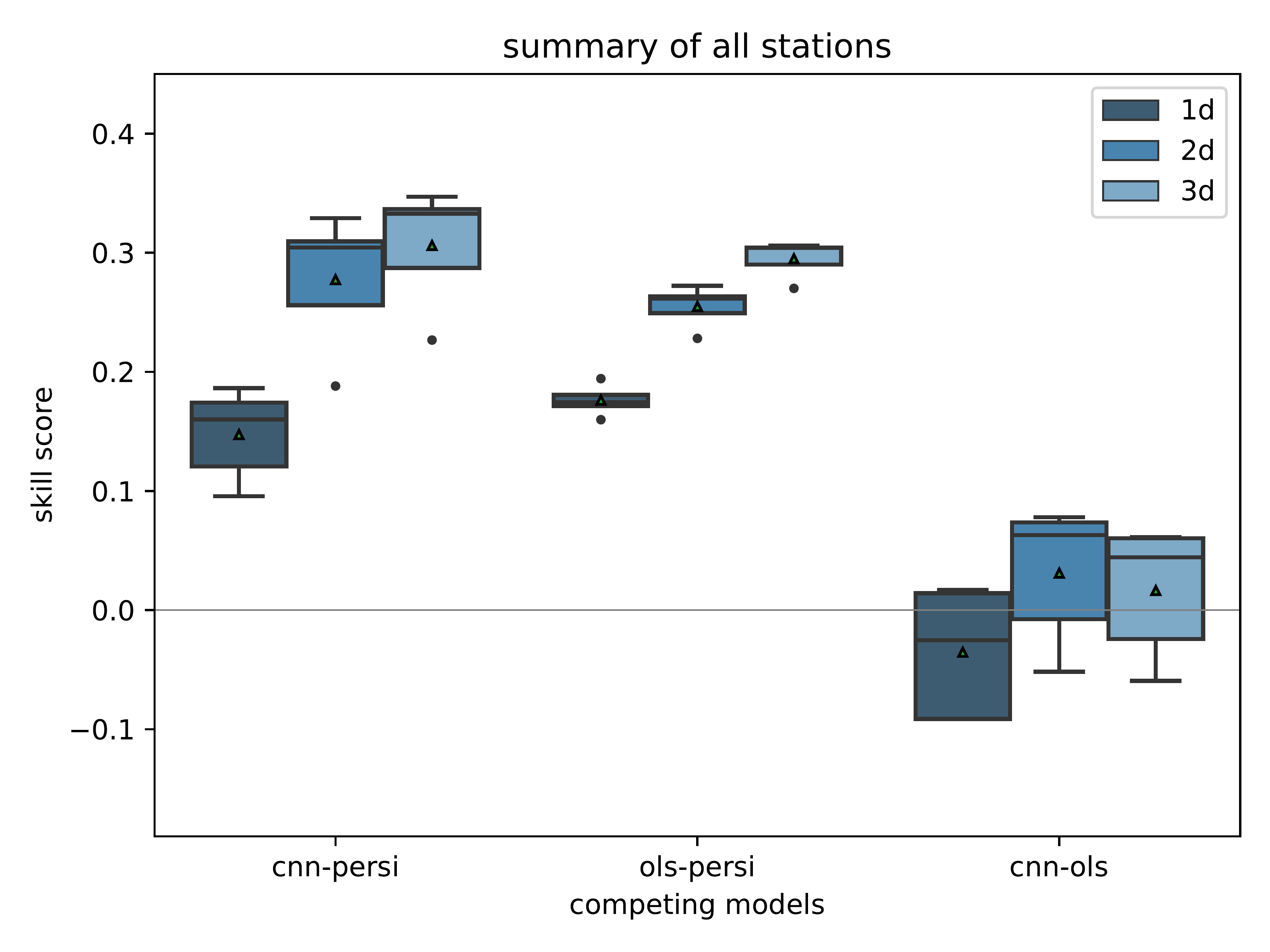
mlair.plotting.postprocessing_plotting.PlotCompetitiveSkillScore(data: Dict[str, pandas.DataFrame], plot_folder='.', model_setup='NN')¶ Bases:
mlair.plotting.abstract_plot_class.AbstractPlotClassCreate competitive skill score plot.
Create this plot for the given model setup and the reference models ordinary least squared (“ols”) and the persistence forecast (“persi”) for all lead times (“ahead”). The plot is saved under plot_folder with the name skill_score_competitive_{model_setup}.pdf and resolution of 500dpi.
- Parameters
data – data frame with index=[‘cnn-persi’, ‘ols-persi’, ‘cnn-ols’] and columns “ahead” containing the pre- calculated comparisons for cnn, persistence and ols.
plot_folder – path to save the plot (default: current directory)
model_setup – architecture type (default “CNN”)
-
_prepare_data(self, data: pandas.DataFrame) → pandas.DataFrame¶ Reformat given data and create plot labels and introduce the dimensions stations and comparison.
- Parameters
data – data frame with index=[‘cnn-persi’, ‘ols-persi’, ‘cnn-ols’] and columns “ahead” containing the pre- calculated comparisons for cnn, persistence and ols.
- Returns
processed data
-
_plot(self, single_model_comparison=False)¶ Plot skill scores of the comparisons.
-
_plot_vertical(self, single_model_comparison=False)¶ Plot skill scores of the comparisons, but vertically aligned.
-
_create_pseudo_order(self, data)¶ Provide first predefined elements and append all remaining.
-
_filter_comparisons(self, data)
-
class
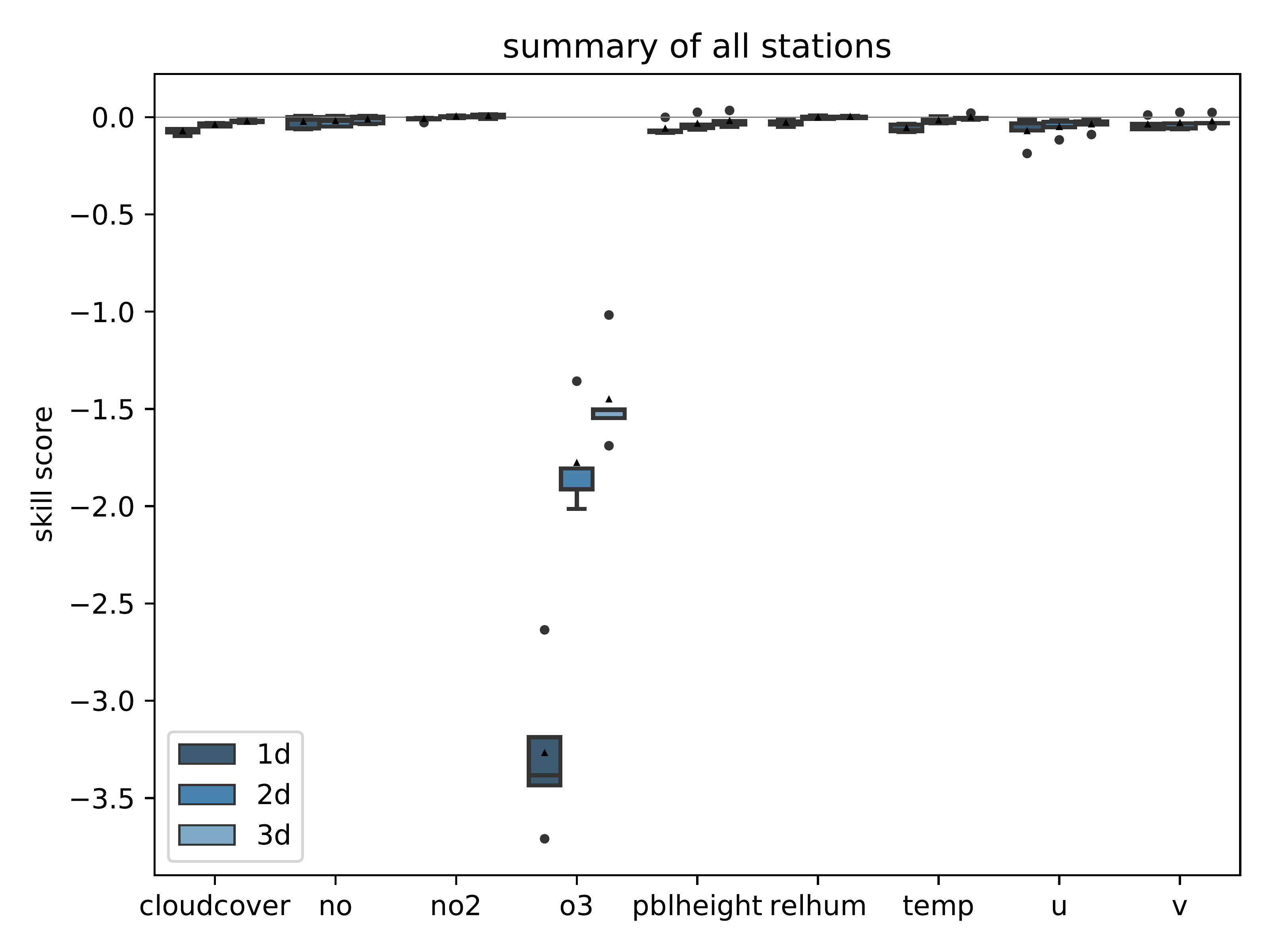
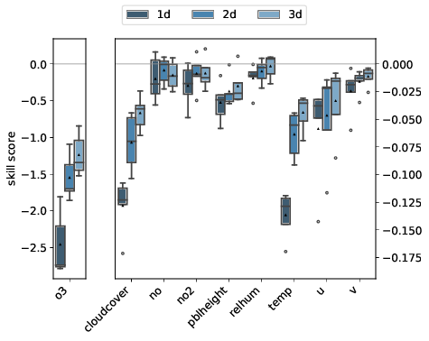
mlair.plotting.postprocessing_plotting.PlotFeatureImportanceSkillScore(data: Dict, plot_folder: str = '.', separate_vars: List = None, sampling: str = 'daily', ahead_dim: str = 'ahead', bootstrap_type: str = None, bootstrap_method: str = None, boot_dim: str = 'boots', model_name: str = 'NN', branch_names: list = None, ylim: tuple = None)¶ Bases:
mlair.plotting.abstract_plot_class.AbstractPlotClassCreate plot of feature importance analysis.
By passing a list separate_vars containing variable names, a second plot is created showing the separate_vars and the remaining variables side by side with different scaling.
-
static
_set_bootstrap_type(boot_type)
-
_set_title(self, model_name, branch=None, n_branches=None)
-
static
_set_bootstrap_method(boot_method)
-
_prepare_data(self, data: Dict, sampling: str) → pandas.DataFrame¶ Shrink given data, if only scores are relevant.
In any case, transform data to a plot friendly format. Also set plot labels depending on the lead time dimensions.
- Parameters
data – dictionary with station names as keys and 2D xarrays as values
- Returns
pre-processed data set
-
_return_vars_without_number_tag(self, values, split_by, keep, as_unique=False)
-
static
_get_number_tag(values, split_by)
-
static
_all_values_are_equal(arr, axis=0)
-
_label_add(self, score_only: bool)¶ Add the phrase “terms and ” if score_only is disabled or empty string (if score_only=True).
- Parameters
score_only – if false all terms are relevant, otherwise only CASE I to IV
- Returns
additional label
-
_plot(self, branch=None, separate_vars=None)¶ Plot climatological skill score.
-
_plot_selected_variables(self, separate_vars: List, branch=None)
-
static
_select_data(df: pandas.DataFrame, variables: List[str], column_name: str) → pandas.DataFrame
-
raise_error_if_vars_do_not_exist(self, data, vars, column_name, name='separate_vars')
-
static
_get_unique_values_from_column_of_df(df: pandas.DataFrame, column_name: str) → List
-
_variables_exist_in_df(self, df: pandas.DataFrame, variables: List[str], column_name: str)
-
_plot_all_variables(self, branch=None)
-
static
-
class
mlair.plotting.postprocessing_plotting.PlotTimeSeries(stations: List, data_path: str, name: str, window_lead_time: int = None, plot_folder: str = '.', sampling='daily', model_name='nn', obs_name='obs', ahead_dim='ahead')¶ Create time series plot.
Currently, plots are under development and not well designed for any use in public.
-
static
_get_sampling(sampling)
-
_get_window_lead_time(self, window_lead_time: int)¶ Extract the lead time from data and arguments.
If window_lead_time is not given, extract this information from data itself by the number of ahead dimensions. If given, check if data supports the give length. If the number of ahead dimensions in data is lower than the given lead time, data’s lead time is used.
- Parameters
window_lead_time – lead time from arguments to validate
- Returns
validated lead time, comes either from given argument or from data itself
-
_load_data(self, station)
-
_plot(self, plot_folder)
-
static
_clean_up_axes(nan_list, axes, fig)
-
static
_save_page(station, pdf_pages)
-
static
_create_plot_data(data, factor, running_index)
-
_create_subplots(self, start, end)
-
_plot_ahead(self, ax, data)
-
_plot_obs(self, ax, data)
-
static
_get_time_range(data)
-
static
-
class
mlair.plotting.postprocessing_plotting.PlotSeparationOfScales(collection: mlair.data_handler.iterator.DataCollection, plot_folder: str = '.', time_dim='datetime', window_dim='window', filter_dim='filter', target_dim='variables')¶ Bases:
mlair.plotting.abstract_plot_class.AbstractPlotClassAbstract class for all plotting routines to unify plot workflow.
Each inheritance requires a _plot method. Create a plot class like:
class MyCustomPlot(AbstractPlotClass):

    def __init__(self, plot_folder, *args, **kwargs):
        super().__init__(plot_folder, "custom_plot_name")
        self._data = self._prepare_data(*args, **kwargs)
        self._plot(*args, **kwargs)
        self._save()

    def _prepare_data(*args, **kwargs):
        <your custom data preparation>
        return data

    def _plot(*args, **kwargs):
        <your custom plotting without saving>
The save method is already implemented in the AbstractPlotClass. If special saving is required (e.g. if you are using pdfpages), you need to overwrite it. Plots are saved as .pdf with a resolution of 500dpi per default (can be set in super class initialisation).
Methods like the shown _prepare_data() are optional. The only method required to implement is _plot.
If you want to add a time tracking module, just add the TimeTrackingWrapper as decorator around your custom plot class. It will log the spent time if you call your plotting without saving the returned object.
@TimeTrackingWrapper
class MyCustomPlot(AbstractPlotClass):
    pass
Let’s assume it takes a while to create this very special plot.
>>> MyCustomPlot()
INFO: MyCustomPlot finished after 00:00:11 (hh:mm:ss)
-
_plot(self, collection: mlair.data_handler.iterator.DataCollection)¶ Abstract plot class needs to be implemented in inheritance.
-
-
class
mlair.plotting.postprocessing_plotting.PlotSampleUncertaintyFromBootstrap(data: xarray.DataArray, plot_folder: str = '.', model_type_dim: str = 'type', error_measure: str = 'mse', error_unit: str = None, dim_name_boots: str = 'boots', block_length: str = None, model_name: str = 'NN', model_indicator: str = 'nn', ahead_dim: str = 'ahead', sampling: Union[str, Tuple[str]] = '', season_annotation: str = None, apply_root: bool = True, plot_name='sample_uncertainty_from_bootstrap')¶ Bases:
mlair.plotting.abstract_plot_class.AbstractPlotClassAbstract class for all plotting routines to unify plot workflow.
Each inheritance requires a _plot method. Create a plot class like:
class MyCustomPlot(AbstractPlotClass):

    def __init__(self, plot_folder, *args, **kwargs):
        super().__init__(plot_folder, "custom_plot_name")
        self._data = self._prepare_data(*args, **kwargs)
        self._plot(*args, **kwargs)
        self._save()

    def _prepare_data(*args, **kwargs):
        <your custom data preparation>
        return data

    def _plot(*args, **kwargs):
        <your custom plotting without saving>
The save method is already implemented in the AbstractPlotClass. If special saving is required (e.g. if you are using pdfpages), you need to overwrite it. Plots are saved as .pdf with a resolution of 500dpi per default (can be set in super class initialisation).
Methods like the shown _prepare_data() are optional. The only method required to implement is _plot.
If you want to add a time tracking module, just add the TimeTrackingWrapper as decorator around your custom plot class. It will log the spent time if you call your plotting without saving the returned object.
@TimeTrackingWrapper
class MyCustomPlot(AbstractPlotClass):
    pass
Let’s assume it takes a while to create this very special plot.
>>> MyCustomPlot()
INFO: MyCustomPlot finished after 00:00:11 (hh:mm:ss)
-
property
get_asteriks_from_mann_whitney_u_result(self)
-
rename_model_indicator(self, data, model_name, model_indicator)
-
prepare_data(self, data: xarray.DataArray)
-
_apply_root(self)
-
_plot_kde(self, agg_type='single', tag='', season='')
-
_plot(self, orientation: str = 'v', apply_u_test: bool = False, agg_type='single', tag='', season='')¶ Abstract plot class needs to be implemented in inheritance.
-
set_significance_bars(self, asteriks, ax, data_table, orientation)
-
property
-
class
mlair.plotting.postprocessing_plotting.PlotTimeEvolutionMetric(data: xarray.DataArray, ahead_dim='ahead', model_type_dim='type', plot_folder='.', error_measure: str = 'mse', error_unit: str = None, model_name: str = 'NN', model_indicator: str = 'nn', time_dim='index')¶ Bases:
mlair.plotting.abstract_plot_class.AbstractPlotClassAbstract class for all plotting routines to unify plot workflow.
Each inheritance requires a _plot method. Create a plot class like:
class MyCustomPlot(AbstractPlotClass):

    def __init__(self, plot_folder, *args, **kwargs):
        super().__init__(plot_folder, "custom_plot_name")
        self._data = self._prepare_data(*args, **kwargs)
        self._plot(*args, **kwargs)
        self._save()

    def _prepare_data(*args, **kwargs):
        <your custom data preparation>
        return data

    def _plot(*args, **kwargs):
        <your custom plotting without saving>
The save method is already implemented in the AbstractPlotClass. If special saving is required (e.g. if you are using pdfpages), you need to overwrite it. Plots are saved as .pdf with a resolution of 500dpi per default (can be set in super class initialisation).
Methods like the shown _prepare_data() are optional. The only method required to implement is _plot.
If you want to add a time tracking module, just add the TimeTrackingWrapper as decorator around your custom plot class. It will log the spent time if you call your plotting without saving the returned object.
@TimeTrackingWrapper
class MyCustomPlot(AbstractPlotClass):
    pass
Let’s assume it takes a while to create this very special plot.
>>> MyCustomPlot()
INFO: MyCustomPlot finished after 00:00:11 (hh:mm:ss)
-
static
_find_nan_edge(data, time_dim)
-
_prepare_data(self, data, time_dim, model_type_dim, model_indicator, model_name)
-
static
_set_ticks(ax, years, months)
-
static
_aspect_cbar(val)
-
_plot(self, data, years, months, vmin=None, vmax=None, subtitle=None)¶ Abstract plot class needs to be implemented in inheritance.
-
_plot_summary_line(self, data, x_dim, y_dim, hue_dim)
-
static
-
class
mlair.plotting.postprocessing_plotting.PlotSeasonalMSEStack(data, data_path: str, plot_folder: str = '.', boot_dim='boots', ahead_dim='ahead', sampling: str = 'daily', error_measure: str = 'MSE', error_unit: str = 'ppb$^2$', time_dim='index', model_type_dim: str = 'type', model_name: str = 'NN', model_indicator: str = 'nn')¶ Bases:
mlair.plotting.abstract_plot_class.AbstractPlotClassAbstract class for all plotting routines to unify plot workflow.
Each inheritance requires a _plot method. Create a plot class like:
class MyCustomPlot(AbstractPlotClass):

    def __init__(self, plot_folder, *args, **kwargs):
        super().__init__(plot_folder, "custom_plot_name")
        self._data = self._prepare_data(*args, **kwargs)
        self._plot(*args, **kwargs)
        self._save()

    def _prepare_data(*args, **kwargs):
        <your custom data preparation>
        return data

    def _plot(*args, **kwargs):
        <your custom plotting without saving>
The save method is already implemented in the AbstractPlotClass. If special saving is required (e.g. if you are using pdfpages), you need to overwrite it. Plots are saved as .pdf with a resolution of 500dpi per default (can be set in super class initialisation).
Methods like the shown _prepare_data() are optional. The only method required to implement is _plot.
If you want to add a time tracking module, just add the TimeTrackingWrapper as decorator around your custom plot class. It will log the spent time if you call your plotting without saving the returned object.
@TimeTrackingWrapper
class MyCustomPlot(AbstractPlotClass):
    pass
Let’s assume it takes a while to create this very special plot.
>>> MyCustomPlot()
INFO: MyCustomPlot finished after 00:00:11 (hh:mm:ss)
-
_prepare_data(self, data)
-
_prepare_data_from_uncertainty(self, boot_dim, data_path, model_type_dim, model_indicator, model_name)
-
static
_set_bar_label(ax)
-
_plot(self, dim, split_ahead=True, sampling='daily', orientation='vertical')¶ Abstract plot class needs to be implemented in inheritance.
-
-
class
mlair.plotting.postprocessing_plotting.PlotErrorsOnMap(data_gen, errors, error_metric, plot_folder: str = '.', iter_dim: str = 'station', model_type_dim: str = 'type', ahead_dim: str = 'ahead', sampling: str = 'daily')¶ Bases:
mlair.plotting.abstract_plot_class.AbstractPlotClassAbstract class for all plotting routines to unify plot workflow.
Each inheritance requires a _plot method. Create a plot class like:
class MyCustomPlot(AbstractPlotClass):

    def __init__(self, plot_folder, *args, **kwargs):
        super().__init__(plot_folder, "custom_plot_name")
        self._data = self._prepare_data(*args, **kwargs)
        self._plot(*args, **kwargs)
        self._save()

    def _prepare_data(*args, **kwargs):
        <your custom data preparation>
        return data

    def _plot(*args, **kwargs):
        <your custom plotting without saving>
The save method is already implemented in the AbstractPlotClass. If special saving is required (e.g. if you are using pdfpages), you need to overwrite it. Plots are saved as .pdf with a resolution of 500dpi per default (can be set in super class initialisation).
Methods like the shown _prepare_data() are optional. The only method required to implement is _plot.
If you want to add a time tracking module, just add the TimeTrackingWrapper as decorator around your custom plot class. It will log the spent time if you call your plotting without saving the returned object.
@TimeTrackingWrapper
class MyCustomPlot(AbstractPlotClass):
    pass
Let’s assume it takes a while to create this very special plot.
>>> MyCustomPlot()
INFO: MyCustomPlot finished after 00:00:11 (hh:mm:ss)
-
static
_calculate_limits(data)
-
static
_set_bounds(limits, ncolors, error_metric)
-
static
_get_colorpalette(error_metric)
-
plot(self, plot_data, error_metric, error_long_name, error_units, model_type, limits, ahead=None)
-
static
_adjust_extent(ax)
-
static
_extract_coords(gen)
-
static
_prepare_data(errors, model_type_dim, model_type, ahead_dim, error_metric, split_ahead=False)
-
static
_draw_background(ax)¶ Draw coastline, lakes, ocean, rivers and country borders as background on the map.
-
_plot_individual(self)
-
static