mlair.plotting.data_insight_plotting

Collection of plots to get more insight into data.

Module Contents

Classes

PlotStationMap	Plot geographical overview of all used stations as squares.
PlotAvailability	Create data availablility plot similar to Gantt plot.
PlotAvailabilityHistogram	Create data availability plots as histogram.
PlotDataMonthlyDistribution	Abstract class for all plotting routines to unify plot workflow.
PlotDataHistogram	Plot histogram on transformed input and target data. This data is the same that the model sees during training. No
PlotPeriodogram	Create Lomb-Scargle periodogram in raw input and target data. The Lomb-Scargle version can deal with missing values.
PlotClimateFirFilter	Plot climate FIR filter components.
PlotFirFilter	Plot FIR filter components.

Functions

f_proc(var, d_var, f_index, time_dim=’datetime’, use_last_value=True)
f_proc_2(g, m, pos, variables_dim, time_dim, f_index, use_last_value)
f_proc_hist(data, variables, n_bins, variables_dim)

Attributes

__author__
__date__

mlair.plotting.data_insight_plotting.__author__ = Lukas Leufen, Felix Kleinert

mlair.plotting.data_insight_plotting.__date__ = 2021-04-13

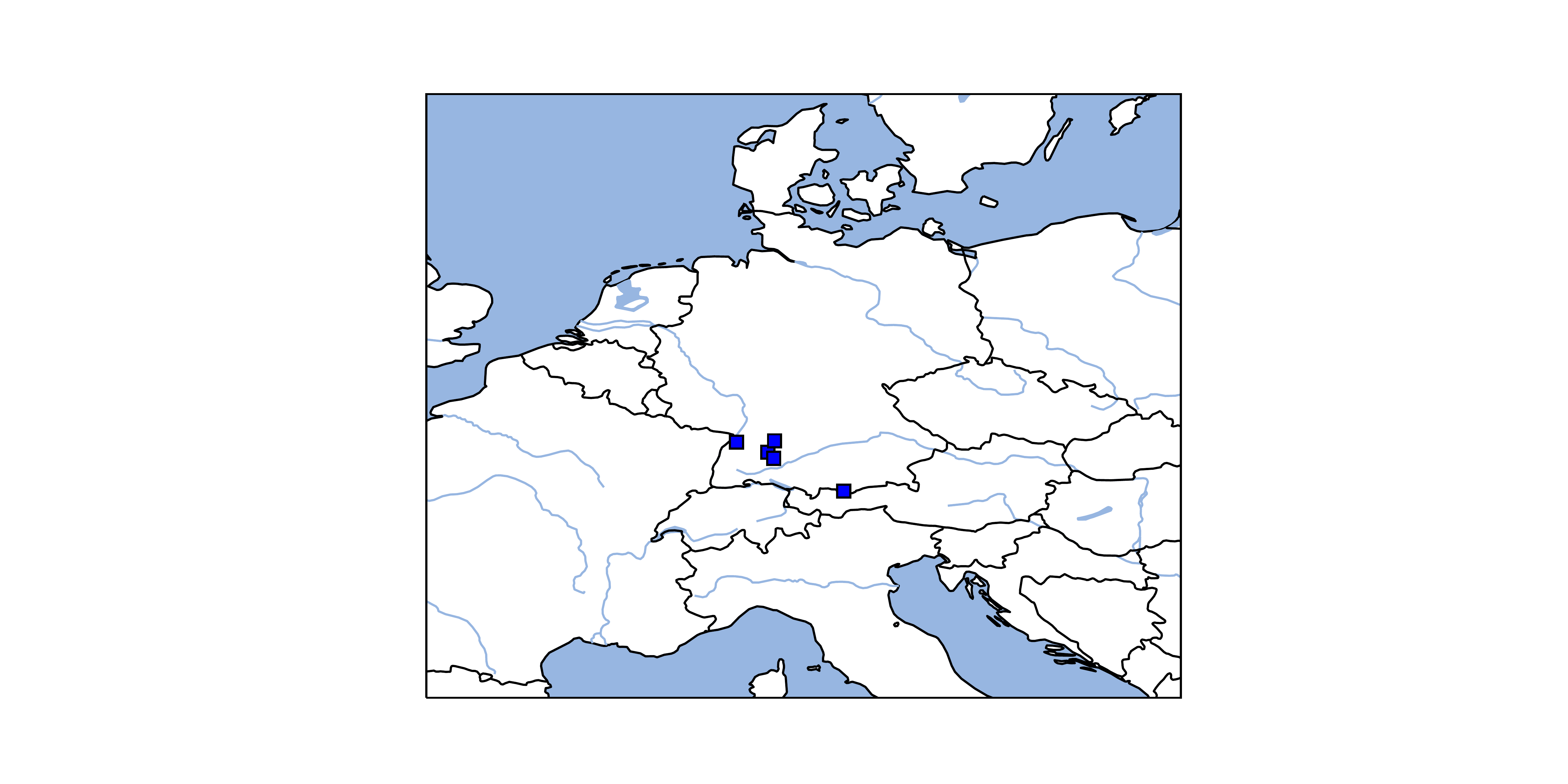
class mlair.plotting.data_insight_plotting.PlotStationMap(generators: List, plot_folder: str = '.', plot_name='station_map')

Bases: mlair.plotting.abstract_plot_class.AbstractPlotClass

Plot geographical overview of all used stations as squares.

Different data sets can be colorised by its key in the input dictionary generators. The key represents the color to plot on the map. Currently, there is only a white background, but this can be adjusted by loading locally stored topography data (not implemented yet). The plot is saved under plot_path with the name station_map.pdf

_draw_background(self)

Draw coastline, lakes, ocean, rivers and country borders as background on the map.

_plot_stations(self, generators)

Loop over all keys in generators dict and its containing stations and plot the stations’s position.

Position is highlighted by a square on the map regarding the given color.

Parameters

generators – dictionary with the plot color of each data set as key and the generator containing all stations as value.

static _adjust_marker(marker)

static _get_collection_and_opts(element)

_plot(self, generators: List)

Create the station map plot.

Set figure and call all required sub-methods.

Parameters

generators – dictionary with the plot color of each data set as key and the generator containing all stations as value.

_adjust_extent(self)

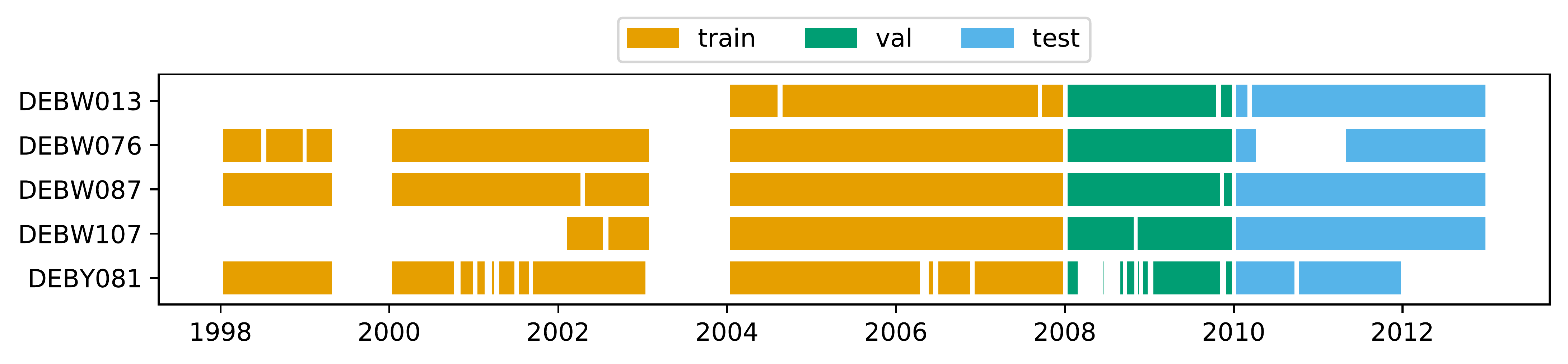
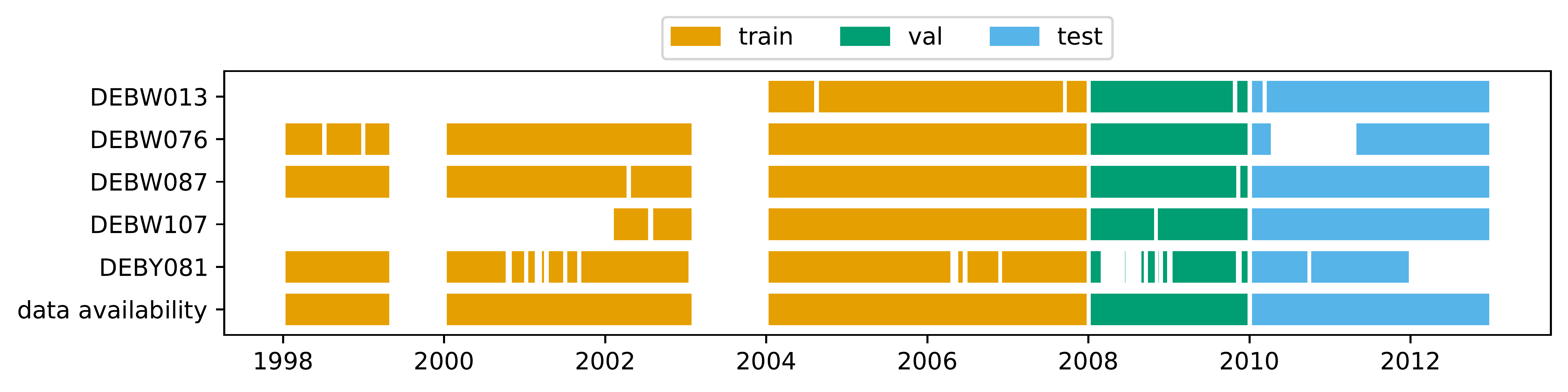
class mlair.plotting.data_insight_plotting.PlotAvailability(generators: Dict[str, mlair.data_handler.DataCollection], plot_folder: str = '.', sampling='daily', summary_name='data availability', time_dimension='datetime', window_dimension='window')

Bases: mlair.plotting.abstract_plot_class.AbstractPlotClass

Create data availablility plot similar to Gantt plot.

Each entry of given generator, will result in a new line in the plot. Data is summarised for given temporal resolution and checked whether data is available or not for each time step. This is afterwards highlighted as a colored bar or a blank space.

You can set different colors to highlight subsets for example by providing different generators for the same index using different keys in the input dictionary.

Note: each bar is surrounded by a small white box to highlight gabs in between. This can result in too long gabs in display, if a gab is only very short. Also this appears on a (fluent) transition from one to another subset.

Calling this class will create three versions fo the availability plot.

1) Data availability for each element 1) Data availability as summary over all elements (is there at least a single elemnt for each time step) 1) Combination of single and overall availability

_prepare_data(self, generators: Dict[str, mlair.data_handler.DataCollection])

_summarise_data(self, generators: Dict[str, mlair.data_handler.DataCollection], summary_name: str)

_plot(self, plt_dict)

Abstract plot class needs to be implemented in inheritance.

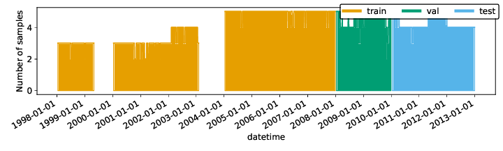
class mlair.plotting.data_insight_plotting.PlotAvailabilityHistogram(generators: Dict[str, mlair.data_handler.DataCollection], plot_folder: str = '.', subset_dim: str = 'DataSet', history_dim: str = 'window', station_dim: str = 'Stations')

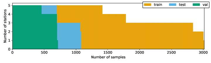
Bases: mlair.plotting.abstract_plot_class.AbstractPlotClass

Create data availability plots as histogram.

Each entry of each generator is checked for notnull() values along all the datetime axis (boolean). Calling this class creates two different types of histograms where each generator

1. data_availability_histogram: datetime (xaxis) vs. number of stations with availabile data (yaxis)

2. data_availability_histogram_cumulative: number of samples (xaxis) vs. number of stations having at least number of samples (yaxis)

_set_dims_from_datahandler(self, data_handler)

property allowed_plot_types(self)

_prepare_data(self, generators: Dict[str, mlair.data_handler.DataCollection])

Prepares data to be used by plot methods.

Creates xarrays which are sums of valid data (boolean sums) across i) station_dim and ii) temporal_dim

_reduce_dims(self, dataset)

static _get_first_and_last_indexelement_from_xarray(xarray, dim_name, return_type='as_tuple')

static _make_full_time_index(irregular_time_index, freq)

_plot(self, plt_type='hist', *args)

Abstract plot class needs to be implemented in inheritance.

_plot_hist(self, *args)

_plot_hist_cum(self, *args)

class mlair.plotting.data_insight_plotting.PlotDataMonthlyDistribution(generators: Dict[str, mlair.data_handler.DataCollection], plot_folder: str = '.', variables_dim='variables', time_dim='datetime', window_dim='window', target_var: str = '', target_var_unit: str = 'ppb')

Bases: mlair.plotting.abstract_plot_class.AbstractPlotClass

Abstract class for all plotting routines to unify plot workflow.

Each inheritance requires a _plot method. Create a plot class like:

class MyCustomPlot(AbstractPlotClass):

    def __init__(self, plot_folder, *args, **kwargs):
        super().__init__(plot_folder, "custom_plot_name")
        self._data = self._prepare_data(*args, **kwargs)
        self._plot(*args, **kwargs)
        self._save()

    def _prepare_data(*args, **kwargs):
        <your custom data preparation>
        return data

    def _plot(*args, **kwargs):
        <your custom plotting without saving>

The save method is already implemented in the AbstractPlotClass. If special saving is required (e.g. if you are using pdfpages), you need to overwrite it. Plots are saved as .pdf with a resolution of 500dpi per default (can be set in super class initialisation).

Methods like the shown _prepare_data() are optional. The only method required to implement is _plot.

If you want to add a time tracking module, just add the TimeTrackingWrapper as decorator around your custom plot class. It will log the spent time if you call your plotting without saving the returned object.

@TimeTrackingWrapper
class MyCustomPlot(AbstractPlotClass):
    pass

Let’s assume it takes a while to create this very special plot.

>>> MyCustomPlot()
INFO: MyCustomPlot finished after 00:00:11 (hh:mm:ss)

_prepare_data(self, generators) → List[xarray.DataArray]

Pre.process data required to plot.

Parameters

generator – data

Returns

The entire data set, flagged with the corresponding month.

static _spell_out_chemical_concentrations(short_name: str, add_concentration: bool = False)

_plot(self, target_var: str, target_var_unit: str)

Create a monthly grouped box plot over all stations but with separate boxes for each lead time step.

Parameters

target_var – display name of the target variable on plot’s axis

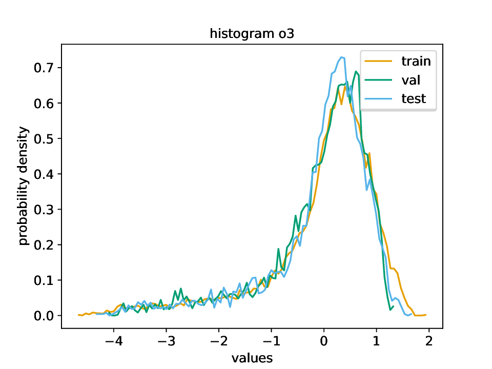
class mlair.plotting.data_insight_plotting.PlotDataHistogram(generators: Dict[str, mlair.data_handler.DataCollection], plot_folder: str = '.', plot_name='histogram', variables_dim='variables', time_dim='datetime', window_dim='window', upsampling=False)

Bases: mlair.plotting.abstract_plot_class.AbstractPlotClass

Plot histogram on transformed input and target data. This data is the same that the model sees during training. No plots are create for the original values space (raw / unformatted data). This plot method will create a histogram for input and target each comparing the subsets train, val and test, as well as a distinct one for the three subsets.

static _handle_upsampling(generators)

static _get_inputs_targets(gens, dim)

_calculate_hist(self, generators, variables, input_data=True, branch_pos=0)

_plot(self, add_name, subset)

Abstract plot class needs to be implemented in inheritance.

_plot_combined(self, add_name)

class mlair.plotting.data_insight_plotting.PlotPeriodogram(generator: Dict[str, mlair.data_handler.DataCollection], plot_folder: str = '.', plot_name='periodogram', variables_dim='variables', time_dim='datetime', sampling='daily', use_multiprocessing=False)

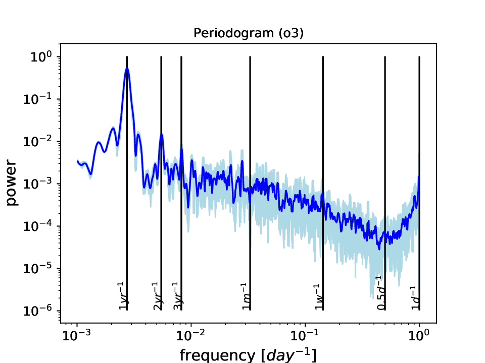
Bases: mlair.plotting.abstract_plot_class.AbstractPlotClass

Create Lomb-Scargle periodogram in raw input and target data. The Lomb-Scargle version can deal with missing values.

This plot routine is creating the following plots:

• “raw”: data is not aggregated, 1 graph per variable

• “”: single data lines are aggregated, 1 graph per variable

• “total”: data is aggregated on all variables, single graph

If data consists on different sampling rates, a separate plot is create for each sampling.

Note

This plot is not included in the default plot list. To use this plot, add “PlotPeriodogram” to the plot_list.

Warning

This plot is highly sensitive to the data handler structure. Therefore, it is highly likely that this method is not compatible with any custom data handler. Proven data handlers are DefaultDataHandler, DataHandlerMixedSampling, DataHandlerMixedSamplingWithFilter. To work properly, the data handler must have the attribute .id_class._data.

static _has_filter_dimension(g, pos)

Inspect if filtered data is provided and return number and labels of filtered components.

_prepare_pgram(self, generator, pos, multiple=1, use_multiprocessing=False, use_last_input_value=True)

Create periodogram data.

_prepare_pgram_parallel_var(self, generator, m, pos, use_multiprocessing)

Implementation of data preprocessing using parallel variables element processing.

_prepare_pgram_parallel_gen(self, generator, m, pos, use_multiprocessing, use_last_input_value=True)

Implementation of data preprocessing using parallel generator element processing.

static _add_annotation_line(ax, pos, div, lims, unit)

_format_figure(self, ax, var_name='total')

Set log scale on both axis, add labels and annotation lines, and set title. :param ax: current ax object :param var_name: name of variable that will be included in the title

_plot(self, raw=True)

Abstract plot class needs to be implemented in inheritance.

_plot_total(self, raw=True)

_plot_difference(self, label_names, plot_name_add='')

mlair.plotting.data_insight_plotting.f_proc(var, d_var, f_index, time_dim='datetime', use_last_value=True)

mlair.plotting.data_insight_plotting.f_proc_2(g, m, pos, variables_dim, time_dim, f_index, use_last_value)

mlair.plotting.data_insight_plotting.f_proc_hist(data, variables, n_bins, variables_dim)

class mlair.plotting.data_insight_plotting.PlotClimateFirFilter(plot_folder, plot_data, sampling, name)

Bases: mlair.plotting.abstract_plot_class.AbstractPlotClass

Plot climate FIR filter components.

• Creates a separate folder climFIR inside the given plot directory.

• For each station up to 4 examples are shown (1 for each season).

• Each filtered component and its residuum is drawn in a separate plot.

• A filter component plot includes the climate FIR input, the filter response, the true non-causal (ideal) filter input, and the corresponding ideal response (containing information about future)

• A filter residuum plot include the climate FIR residuum and the ideal filter residuum.

_prepare_data(self, data)

Restructure plot data.

_plot(self, plot_dict, sampling, new_dim='window')

Abstract plot class needs to be implemented in inheritance.

static _set_ylim_by_valid_range(ax, a, b, dim, valid_range)

_set_xlim(self, ax, t0, order, valid_range, td_type, time_axis)

Set xlims

Use order and valid_range to find a good zoom in that hides edges of filter values that are effected by reduced filter order. Limits are returned to be usable for other plots.

_plot_valid_area(self, ax, t0, valid_range, td_type)

_plot_t0(self, ax, t0)

_plot_series(self, ax, time_axis, data, style)

_plot_original_data(self, ax, time_axis, data)

_plot_apriori(self, ax, time_axis, data, new_dim, ifilter, offset)

_plot_clim_filter(self, ax, time_axis, data, new_dim, h, output_dtypes)

_plot_ideal_filter(self, ax, time_axis, data, new_dim, h, output_dtypes)

_store_plot_data(self, data)

Store plot data. Could be loaded in a notebook to redraw.

class mlair.plotting.data_insight_plotting.PlotFirFilter(plot_folder, plot_data, name)

Bases: mlair.plotting.abstract_plot_class.AbstractPlotClass

Plot FIR filter components.

• Creates a separate folder FIR inside the given plot directory.

• For each station up to 4 examples are shown (1 for each season).

• Each filtered component and its residuum is drawn in a separate plot.

• A filter component plot includes the FIR input and the filter response

• A filter residuum plot include the FIR residuum

_prepare_data(self, data)

Restructure plot data.

_plot(self, plot_dict)

Abstract plot class needs to be implemented in inheritance.

_plot_t0(self, ax, t0)

_plot_series(self, ax, time_axis, data, style)

_plot_data(self, ax, time_axis, data, style='original')

_store_plot_data(self, data)

Store plot data. Could be loaded in a notebook to redraw.